Esprit des Pyrénées

Day One: Introduction

This blog is a reflection of my inner mathematical monologue. It will host discussions of: my current research and interests, talks and seminars that I have given or attended, and various problems that I think are interesting. I am no longer in academia, but I am very much so still involved in the general sphere of mathematics education.

Berge-Kang primitive/Seifert-fibered knot; drawing by me, editing and color-enhancements by Chloe Hsu

Two Problems.

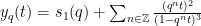
Let $N$ be any natural number, and suppose $N = \prod_{i=1}^n p_i^{e_i}$ be its prime factorization. WLOG assume that $p_1 > p_2 > \cdots p_n$ . From this data we can associate two quantities to $N$ :
$\alpha(N) = \frac{\sum_{i=1}^n e_ip_i}{\sum_{i=1}^n e_i},$
and
$\beta(N) = p_1 - \frac{1}{p_1-\frac{1}{\ddots - \frac{1}{p_2 - \frac{1}{\ddots - \frac{1}{p_n - \frac{1}{\ddots - \frac{1}{p_n}}}}}}}.$
where $p_i$ appears $e_i$ times in the continued fraction.

Prove or find a counter-example: if $N$ is not prime and $\alpha(N) = \beta(N),$ then $N = 2^e \cdot 3$ for some exponent $e\geq 1.$
The “factorial” triple problem is a fascinating topic in number theory. We say that a triplet of natural numbers $(a,b,c)$ is a factorial triple if $a!\cdot b! = c!$ Obviously there are the “trivial” examples $n!(n!-1)! = (n!)!$ just using the definition of factorial. Also, if $a$ or $b$ is equal to $1,$ then the equation is vacuous. There is one known “nontrivial” solution to this equation; namely $6!\cdot 7! = 10!$ This problem has been relatively well-studied; however, here is a slight generalization of it: we define the $k$ -fold multifactorial of $n$ as
$n\overset{k}{!} = \prod_{\substack{d = 1 \\ d\equiv n\pmod k}}^n d.$
In other words, $n\overset{k}!$ is the product of all integers from $1$ to $n$ that are congruent to $n$ mod $k.$ Now we can consider the $k$ -fold analogue of the factorial triple problem: $a\overset{k}{!}\cdot b\overset{k}{!} = c\overset{k}{!}$ Notice if $g > \max\{a,b,c\},$ then the equation degenerates to $a\cdot b = c.$ This equation has tons of solutions (just look at the divisors of $c$ )!

Find a family or prove finiteness: for some $1 < k << \infty,$ find a family of solutions to $a\overset{k}{!}\cdot b\overset{k}{!} = c\overset{k}{!}$

Tate Uniformization

Here I will review Tate’s uniformization of Elliptic curves over ${{\mathbb C}}$ and over ${p}$ –adic fields. Historically, Tate’s work served as motivation for Mumford’s uniformization of ${p}$ –adic hyperbolic curves, which I plan on discussing in a subsequent post. If ${E}$ is an elliptic curve defined over ${{\mathbb C}}$ , the full Uniformization Theorem of Riemann surfaces implies that ${E({\mathbb C}) \cong {\mathbb C}/({\mathbb Z}\oplus {\mathbb Z}\tau)}$ , where ${{\mathbb Z}\oplus {\mathbb Z}\tau}$ is a lattice inside ${{\mathbb C}}$ . Without loss of generality assume ${\mathrm{Im}(\tau) > 0}$ . By factoring the quotient, note that ${E({\mathbb C})\cong \left({\mathbb C}/{\mathbb Z}\right)/{\mathbb Z}\tau}$ . 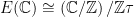Consider the analytic isomorphism ${\mathrm{exp}: {\mathbb C}/{\mathbb Z}\rightarrow {\mathbb C}^{\times}}$ given by the exponential map ${z\mapsto e^{2\pi i z}}$ . Define ${q = e^{2\pi i \tau}}$ and ${q^{{\mathbb Z}} = \{q^n : n\in {\mathbb Z}\}}$ . Observe that ${|q| < 1}$ . Moreover observe that ${\mathrm{exp}}$ induces an analytic isomorphism
$\displaystyle \left({\mathbb C}/{\mathbb Z}\right)/{\mathbb Z}\tau \xrightarrow{\sim} {\mathbb C}^{\times}/q^{{\mathbb Z}}$

given by ${z \mapsto e^{2\pi i z}}$ . In fact, we can give an explicit analytic description of the resulting isomorphism ${E({\mathbb C})\cong {\mathbb C}^{\times}/q^{{\mathbb Z}}}$ using q-expansions: set ${s_k = \sum_{n\geq 1} \frac{n^k q^n}{1-q^n}}$ , ${a_4 = -5s_3(q)}$ , ${a_6(q) = \frac{a_4(q) - 7s_5(q)}{12}}$ , ${x_q(t) = -2s_1(q) + \sum_{n\in {\mathbb Z}} \frac{q^nt}{(1-q^nt)^2}}$ , and ${y_q(t) = s_1(q) + \sum_{n\in {\mathbb Z}} \frac{(q^nt)^2}{(1-q^nt)^3}}$ .

Theorem 1 If ${q \in {\mathbb C}^{\times}}$ and ${|q|<1}$ , then there exists a complex elliptic curve ${E_q}$ and a complex–analytic isomorphism
$\displaystyle {\mathbb C}^{\times}/q^{{\mathbb Z}} \xrightarrow{\sim} E_q({\mathbb C})$

Proof: Let ${E_q}$ denote the curve cut out by the Weierstrass equation

$\displaystyle E_q: y^2+xy = x^3 + a_4(q)x + a_6(q)$

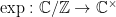
and define the map in the Theorem by
$\displaystyle t \mapsto \begin{cases} (x_q(t),y_q(t)) & e^{2\pi i z} \not\in q^{{\mathbb Z}} \\ P & e^{2\pi i z}\in q^{{\mathbb Z}} \end{cases}$

where ${P}$ indicates a fixed origin point on ${E_q}$ . A full proof of the Theorem can be found in Silverman’s second book on elliptic curves. $\Box$

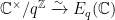
The ability to compute cohomological invariants of curves is one of the main applications of classical uniformization theories. So when one studies the ${l}$ –adic cohomology of ${p}$ –adic abelian varieties, a natural question that arises is if there exists an analogue of Theorem~1. Let ${K}$ be a complete non–archimedian field of residue characteristic ${p}$ with ring of integers ${{\cal O}_K}$ and maximal ideal ${m}$ . If one tries to generalize the usual description of elliptic curves as the quotient of ${{\mathbb C}}$ by some lattice, issues quickly arise. First of all, ${K}$ is totally disconnected with respect to its natural topology. So the notion of analyticity becomes more complicated. This issue is resolved by passing to the rigid–analytic, or more generally, the adic category. Additionally, when ${K}$ is mixed characteristic, ${K}$ does not contain non-trivial discrete subgroups. And when ${K}$ is of characteristic ${(p,p)}$ , then such subgroups may exist, but their quotients do not define Abelian varieties. The latter phenomena leads to the study of Drinfeld modules, which is an incredible subject in its own right (and I may dedicate a future blog post to it). Nevertheless, Tate’s insight was that ${K^{\times}}$ contains non-trivial lattices: for any ${q\in K^{\times}}$ with ${|q|< 1}$ , ${q^{{\mathbb Z}}}$ is a discrete subgroup in ${K^{\times}}$ . So one might hope that the uniformization in Theorem~1 can be generalized to the ${p}$ –adic setting. This is indeed the case.

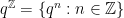
Theorem 2 (Tate) For each ${q \in K^{\times}}$ with ${|q| < 1}$ , there exists an elliptic curve ${E_q}$ over ${K}$ such that ${\mathbb{G}_m^{an}/q^{{\mathbb Z}} \xrightarrow{\sim} E_q^{an}}$ is an isomorphism of rigid–analytic spaces. In particular, ${L^{\times}/q^{{\mathbb Z}} \cong E_q(L)}$ is an isomorphism for each algebraic extension ${L}$ of ${K}$ , which is ${\mathrm{Gal}(L/K)}$ –equivariant whenever ${L}$ is Galois over ${K}$ .

Proof: In fact, one defines ${E_q}$ using the same formula as in Theorem~1. The point being that ${a_4}$ and ${a_6}$ define ${p}$ –adically convergent series. The analytic structure of ${E_q}$ was originally formulated in terms of rigid–analytic spaces. Recall that ${\mathbb{G}_{m} = \text{Spec }K[T,U]/(TU - 1) = \text{Spec }K[T,T^{-1}]}$ . Then the rigid–analytification of ${\mathbb{G}_{m}}$ is given by the base space ${\mathbb{G}_{m}^{an} = \text{Spm }K/(TU - 1) = \text{Spm }K}$ together with the Grothendieck topology of admissible covers ${\{U_n\}_{n\geq 0}}$ , where ${U_n = \{z\in K^{\times}: |q|^{\frac{n+1}{2}}< |z|< |q|^{\frac{n}{2}}\} = \text{Spm }K<T,T^{-1},X,Y>/(TY - q^{\frac{n+1}{2}}, T - |q|^{\frac{n}{2}}X)}$ , ${\text{Spm}}$ denotes the maximal spectrum, and ${K<T,U>}$ is the Tate algebra in two variables. Note that ${q}$ acts on the ${U_n}$ discontinuously via ${U_n\mapsto U_{n+2}}$ , so the quotient ${\mathbb{G}_m^{an}/q^{{\mathbb Z}}}$ is a well defined rigid–analytic space covered by the images of ${U_0}$ and ${U_1}$ . One then shows that ${\mathbb{G}_m^{an}/q^{{\mathbb Z}}}$ is isomorphic to ${E_q^{an}}$ . The full proof can be found in Tate’s article A review of non-Archimedean elliptic functions. $\Box$

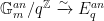
The situation for higher–dimensional abelian varieties is similar. Consider ${(\mathbb{G}_m^{an})^g = \text{Spm }K<T_1,T_1^{-1},\dots ,T_g,T_g^{-1}>}$ and note there exists a natural group homomorphism ${{\cal L}: (\mathbb{G}_m^{an})^g \rightarrow {\mathbb R}^g}$ given by ${{\cal L}(z) = (-\log|z_1|,\dots,-\log|z_g|)}$ . We say that ${\Lambda}$ is a lattice in ${(\mathbb{G}_m^{an})^g}$ if ${{\cal L}(\Lambda)}$ is a lattice in ${{\mathbb R}^g}$ . It can be shown that ${(\mathbb{G}_m^{an})^g/\Lambda}$ then has the structure of a rigid–analytic space that is also an abelian variety.

Uniformization of Complex Hyperbolic Curves

I do not intend to prove any results in this post, but for the sake of exposition as I work towards understaning Mochizuki’s ${p}$ –adic uniformization theory, I would like to review the uniformization of complex–analytic hyperbolic curves. There are three main ways to realize such curves as the quotient of a topological space by the action of some group that acts discontinuously. We will focus primarily on the first two uniformizations described below.

Let ${\mathop{\mathbb H}^2}$ (resp. ${\mathop{\mathbb H}^3}$ ) denote the upper–half plane (resp. hyperbolic 3–space), and denote ${\mathop{\mathbb H}^2\sqcup \partial \mathop{\mathbb H}^2 = \mathop{\mathbb H}^2\sqcup \mathop{\mathbb P}^1{\mathbb R}}$ (resp. ${\mathop{\mathbb H}^3\sqcup \partial \mathop{\mathbb H}^3 = \mathop{\mathbb H}^3\sqcup \mathop{\mathbb P}^1{\mathbb C}}$ ) by ${\overline{\mathop{\mathbb H}^2}}$ (resp. ${\overline{\mathop{\mathbb H}^3}}$ ) . Let ${X}$ be a ${r}$ –punctured genus ${g}$ curve over ${{\mathbb C}}$ such that ${2g-2+r > 0}$ (i.e has negative Euler characteristic and admits a hyperbolic structure). A hyperbolic structure on ${X}$ is, by definition, a choice of an atlas ${\{U_i\}}$ on ${X}$ with transition maps ${U_i\xrightarrow{\phi_i} \mathop{\mathbb H}^2\xrightarrow{\phi_j^{-1}} U_j\cap U_i}$ . We take as fact that such a choice induces an isometry ${\widetilde{X}\cong \mathop{\mathbb H}^2}$ , where ${\widetilde{X}}$ is the universal cover of ${X}$ .

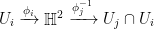
Fuchsian–Koebe Uniformization: The group ${\mathrm{PSL}_2({\mathbb R})}$ acts transitively on ${\mathop{\mathbb H}^2}$ via fractional linear transformations:
$\displaystyle \left[\begin{smallmatrix} a & b \\ c & d \end{smallmatrix}\right]\cdot z \mapsto \frac{az+b}{cz+d}$

In fact, ${\mathrm{Aut}(\overline{\mathop{\mathbb H}^2}) \cong \mathrm{PSL}_2({\mathbb R})}$ . It follows that the identification ${\widetilde{X}\cong \mathop{\mathbb H}^2}$ induces a representation
$\displaystyle \rho_X: \pi_1(X)\rightarrow \mathrm{PSL}_2({\mathbb R})$

which is sometimes called the canonical representation. Set ${\Gamma_F = \rho_X(\pi_1(X))}$ . The resulting isometry
$\displaystyle X \cong \mathop{\mathbb H}^2/\Gamma_F$

is called the Fuchsian–Koebe uniformization of ${X}$ .

Schottky Uniformization: Observe that ${\rho_X}$ gives a natural ${\mathrm{PSL}_2({\mathbb C})}$ –representation after composition with the inclusion ${\mathrm{PSL}_2({\mathbb R})\rightarrow \mathrm{PSL}_2({\mathbb C})}$ . Moreover, we may compactify ${X}$ by ordering and filling its set of punctures so that they are viewed as marked points. Let ${X' = \overline{\mathop{\mathbb H}^2}/\Gamma_F}$ denote the compactification of ${X}$ . Topologically speaking, ${r}$ –pointed and ${r}$ –punctured curves carry the same information and define the same point in the relevant moduli stack. The distinction between ${X}$ and ${X'}$ becomes necessary when discussing uniformization. Now recall from the post “Cusps on Bianchi Orbifolds I”, the group ${\mathrm{PSL}_2({\mathbb C})}$ acts on ${\overline{\mathop{\mathbb H}^3}}$ by Poincaré extending the fractional linear transformation on the sphere at ${\infty}$ to all of ${\mathop{\mathbb H}^3}$ . Formulaically,
$\displaystyle \left[\begin{smallmatrix} a & b \\ c & d \end{smallmatrix}\right]\cdot (z,t) \mapsto \left(\frac{\overline{(cz + d)}(az+b) + a\overline{c}t^2}{|cz+d|^2 + |c|^2t^2},\frac{t}{|cz+d|^2 + |c|^2t^2}\right)$

Similar to the case in two dimensions, one can show that ${\mathrm{Aut}(\mathop{\mathbb H}^3) \cong \mathrm{Aut}(\mathop{\mathbb P}^1{\mathbb C})\cong \mathrm{PSL}_2({\mathbb C})}$ .

Suppose that ${\Gamma_S}$ is a free, finitely generated Kleinian group that consists only of loxodromic elements: see Cusps on Bianchi Orbifolds I for the classification of Möbius transformations. A Theorem of Maskit in A Characterization of Schottky Groups implies that ${\Gamma_S}$ acts discontinuously on some nonempty connected domain ${D(\Gamma_S)\subset \mathop{\mathbb P}^1{\mathbb C}}$ bounded by ${2g}$ Jordan curves ${A_1,B_1,\dots A_g,B_g}$ whose interiors are pairwise disjoint and such that for each ${i}$ there exists ${\gamma_i\in \Gamma_S}$ with the properties ${\gamma_i(A_i) = B_i}$ and ${\gamma_i(D(\Gamma_S))\cap D(\Gamma_S) = \emptyset}$ . Any such ${\Gamma_S}$ is known as a Schottky group and any domain in ${\mathop{\mathbb P}^1{\mathbb C}}$ that is the maximal connected locus of discontinuity for the action of some Schottky group is called a Schottky domain. Set ${\overline{D} = D\cup \bigcup_i \left(A_i\cup B_i\right)}$ and let ${\Omega(\Gamma_S) = \bigcup_{\gamma\in \Gamma_S}\gamma(\overline{D})}$ denote the full locus of discontinuity for the action of ${\Gamma_S}$ . The condition that all elements are loxodromic is equivalent to ${\Gamma_S}$ containing no unipotent, i.e parabolic, elements. Passing to the quotient, one obtains homeomorphisms
$\displaystyle (\mathop{\mathbb H}^3\sqcup \Omega)/\Gamma_S \simeq \Theta_g$

and
$\displaystyle \omega:\Omega(\Gamma_S)/\Gamma_S \simeq \partial\Theta_g = \Sigma_g$

where ${\Theta_g}$ denotes the Handlebody obtained by attaching ${g}$ handles to a solid torus, and ${\Sigma_g}$ denotes the boundary surface of genus ${g}$ . Intuitively, the ${2g}$ boundary components of ${D(\Gamma_S)}$ are identified in pairs via the action of ${\Gamma_S}$ , and the base solid torus of ${\Theta_g}$ manifests in the Poincaré extension of the ${\Gamma_S}$ –action to ${\mathop{\mathbb H}^3}$ . Note that ${\Sigma_g}$ is compact, ergo closed. The hyperbolic metric on ${\overline{\mathop{\mathbb H}^3}}$ induces a hyperbolic structure on ${\Sigma_g}$ , so ${\omega}$ can be promoted to an isometry of Riemann surfaces. The description of ${\Sigma_g}$ as the quotient ${\Omega(\Gamma_S)/\Gamma_S}$ is called the Schottky uniformization of ${\Sigma_g}$ .

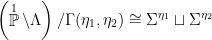
It turns out that every closed Riemann surface of genus ${g > 1}$ admits a Schottky uniformization; however, the closedness condition excludes punctured surfaces. There is a way to handle surfaces with an even number of punctures, using so–called extended Schottky groups, but we will not discuss these here. Instead, we consider marked surfaces. This will allow us to relate the Fuchsian–Koebe and Schottky uniformizations on the level of covering maps and fundamental groups.

Suppose ${\Gamma_S}$ is free on generators ${\gamma_1,\dots, \gamma_g}$ . A marked Schottky group is a Schottky group equipped with an ordered choice of free generators. Let ${{\cal S}_g}$ denote the moduli space of marked Schottky groups of genus ${g}$ . ${{\cal S}_g}$ consists of classes, under Möbius transformation, of ordered ${g}$ –tuples that generate a Schottky group. Let ${{\cal S}_{g,r}}$ denote the holomorphic fibration over ${{\cal S}_g}$ whose fiber over a point ${[\Gamma_S] \in {\cal S}_g}$ is the configuration spaces of ${r}$ –points on ${\Omega(\Gamma_S)/\Gamma_S}$ . ${{\cal S}_{g,r}}$ can be thought of as the space of equivalence classes of tuples ${(\Gamma_S, \Omega(\Gamma_S)/\Gamma_S, \{s_1,\dots, s_r\})}$ , where the ${s_i}$ indicate marked points on ${\Omega(\Gamma_S)/\Gamma_S}$ . Note that the ${s_i}$ define a ${\Gamma_S}$ –orbit of points, whose representatives are also denoted ${s_i}$ , in ${\Omega(\Gamma_S)\subset \mathop{\mathbb P}^1{\mathbb C}}$ . Fix ${(\Gamma_S, \Omega(\Gamma_S)/\Gamma_S, \{s_1,\dots, s_r\})\in {\cal S}_{g,r}}$ , set ${X' = \Omega(\Gamma_S)/\Gamma_S}$ , and let ${X = X'\backslash\{s_1,\dots,s_r\}}$ . Then ${X = \mathop{\mathbb H}^2/\Gamma_F}$ for some Fuchsian goup ${\Gamma_F < \mathrm{PSL}_2({\mathbb R})}$ . Let ${\overline{\mathop{\mathbb H}^2}_{\Gamma_F}}$ denote the union of ${\mathop{\mathbb H}^2}$ with the cusps of ${\Gamma_F}$ and recall that the ${j}$ –invariant defines a bijective Hauptmodul
$\displaystyle j: X \rightarrow \mathop{\mathbb P}^1\backslash\{p_1,\dots, p_r\}$

for some points ${p_i\in \mathop{\mathbb P}^1{\mathbb C}}$ . Without loss of generality assume that ${p_i = s_i}$ for each ${i=1,\dots, r}$ . Note that ${j}$ lifts to a bijection
$\displaystyle \overline{j}: \overline{\mathop{\mathbb H}^2}_{\Gamma_F}/\Gamma_F \rightarrow \mathop{\mathbb P}^1{\mathbb C}$

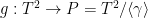
that sends the ${\Gamma_F}$ –orbit of the ${\{x_i\}}$ to the ${\Gamma_S}$ –orbit of ${\{s_i\}}$ . In particular, after restricting the codomain, lifting the domain to ${\overline{\mathop{\mathbb H}^2}_{\Gamma_F}}$ , and then composing with ${\omega}$ , one obtains covering maps
$\displaystyle \overline{\mathop{\mathbb H}^2}_{\Gamma_F}\rightarrow \Omega(\Gamma_S)\rightarrow \Sigma_g$

Suppose ${\Gamma_F = \pi_1(\Sigma_g)}$ is generated by a standard meridian–longitude basis ${\mu_1,\lambda_1,\dots,\mu_g,\lambda_g}$ , and let ${N_{\mu}}$ denote the smallest normal subgroup of ${\Gamma_F}$ containing ${\mu_1,\dots,\mu_g}$ . One can show that ${\omega}$ is the topological covering space corresponding to the subgroup ${N_{\mu}}$ . From ${\omega}$ and the Fuchsian uniformization ${\overline{\mathop{\mathbb H}^2}_{\Gamma_F}/\Gamma_F\rightarrow \Sigma_g}$ it follows that
$\displaystyle \Gamma_S = \Gamma_F/N_{\mu}$

Bers (Simultaneous) Uniformization: We conclude this discussion by mentioning the Bers simultaneous uniformization Theorem, which looks similar to the Schottky uniformization, but applies to a compact Riemann surface ${\Sigma}$ that admits two hyperbolic structures ${\eta_1}$ and ${\eta_2}$ . We call a Kleinian group ${\Gamma}$ quasi–Fuchsian of type I if its limit set ${\Lambda \subset \mathop{\mathbb P}^1{\mathbb C}}$ is equal to a ${\Gamma}$ –invariant Jordan curve.

Theorem 1: If a compact Riemann surface ${\Sigma}$ admits hyperbolic structures ${\eta_1}$ and ${\eta_2}$ , then there exists a quasi–Fuchsian group of type I ${\Gamma(\eta_1,\eta_2)}$ such that
$\displaystyle \left(\mathop{\mathbb P}^1\backslash \Lambda\right)/\Gamma(\eta_1,\eta_2) \cong \Sigma^{\eta_1}\sqcup \Sigma^{\eta_2}$

where ${\Lambda}$ is the invariant Jordan curve of ${\Gamma(\eta_1,\eta_2)}$ and ${\Sigma^{\eta_i}}$ indicates ${\Sigma}$ equipped with the hyperbolic structure ${\eta_i}$ .

The main observation towards proving such a result is that ${\Lambda}$ divides ${\mathop{\mathbb P}^1{\mathbb C}}$ into two open discs ${\Omega_1}$ and ${\Omega_2}$ , each of which is conformally equivalent to ${\mathop{\mathbb H}^2}$ . So it suffices to find Fuchsian groups ${\Gamma_1}$ and ${\Gamma_2}$ such that ${\Omega_i/\Gamma(\eta_1,\eta_2)\cong \mathop{\mathbb H}^2/\Gamma_i}$ .

Cusps on Bianchi Orbifolds II

I need to clarify a minor mistake (now corrected) that was made out of haste in my previous post. Thankfully this leads nicely into a discussion that I was planning on writing about anyways. Recall the following result from part I (Lemma 8):

Lemma 1: If ${M}$ is an orientable hyperbolic 3–orbifold of finite volume, then ${M}$ has finitely many ends (i.e. cusp neighborhoods) and each end is isometric to ${\widetilde{T}\times [0,\infty)}$ , where ${\widetilde{T}}$ is some quotient of the 2–torus ${T^2}$ . Moreover, the stabilizer subgroup of each cusp ${{\mathbb Z}\oplus {\mathbb Z}}$ , generated by a pair of parabolics.

Before the correction, I had written that the cusp neighborhoods are isometric to ${T^2\times [0,\infty)}$ . As the proof of the above Lemma implies, this is true if and only if the covering group ${\Gamma}$ does not contain torsion elements that fix the point at ${\infty}$ . The existence of such elements introduces interesting delicacies that are relevant to some of the problems I have been working on. In general, if there are elliptic elements that fix a cusp at ${\infty}$ , then the cusp is called rigid. This means that it cannot be deformed; and in particular, Dehn surgery cannot be performed (unless the cusp is ${S^2(2,2,2,2)}$ ). We will explain and investigate these last statements in a later post when we discuss arithmetic knot complements (Cusps on Bianchi Orbifolds III).

Assume from here-on-out that ${\Gamma = \Gamma_d = \mathrm{PSL}_2({\cal O}_d)}$ is a Bianchi group. Then the number of cusps on ${\mathop{\mathbb H}^3/\Gamma_d}$ is equal to the class number of ${K_d}$ , so there is always at least one cusp. In what follows we will show that the cusp cross sections of ${\mathop{\mathbb H}^3/\Gamma_d}$ are tori unless ${d \in \{1,3\}}$ . Moreover, unless ${d = 3}$ , all cusp cross sections are non–rigid.

Lemma 2: If ${\gamma \in \mathrm{PSL}_2({\mathbb C})}$ has finite order, then ${\gamma}$ is an elliptic Möbius transformation.

Proof: Suppose ${\gamma^k = \left[\begin{smallmatrix} 1 & \\ & 1 \end{smallmatrix}\right]}$ for some positive integer ${k}$ . Observe that ${\gamma}$ is not conjugate to a matrix of the form ${\left[\begin{smallmatrix} 1 & \alpha \\ & 1 \end{smallmatrix}\right]}$ for some complex number ${\alpha}$ since otherwise ${\gamma}$ would be parabolic, hence have infinite order. So ${\gamma}$ has two distinct fixed points on ${{\mathbb C}}$ , therefore is conjugate to a marix of the form ${\left[\begin{smallmatrix} \lambda & \\ & \lambda^{-1} \end{smallmatrix}\right]}$ . It is an elementary group–theoretic fact that conjugates of torsion elements are also torsion, which implies that ${\lambda^k = 1}$ . It follows that ${\lambda}$ is a root of unity, so ${\lambda + \lambda^{-1}}$ is real and ${|\lambda + \lambda^{-1}|}$ is less than ${2}$ . Since the square trace map is invariant under conjugation. and the trace is invariant up to multiplication by ${-1}$ , we conclude that ${\gamma}$ is elliptic. $\Box$

The Dirichlet Unit Theorem implies that the group of units in any imaginary quadratic field has rank ${0}$ . Hence any unit in ${{\cal O}_d}$ is a root of unity. It turns out that the existence of such elements is rare, as the following Lemma shows.

Lemma 3: ${{\cal O}_d}$ contains a non-real root of unity if and only if ${d \in \{1,3\}}$ .

Proof: The “if” direction is clear given the element ${i \in {\cal O}_1}$ and ${\zeta_3 = \frac{1+\sqrt{-3}}{2}}$ in ${{\cal O}_3}$ . Conversely, suppose ${{\cal O}_d}$ contains an ${n^{th}}$ –root of unity ${\zeta_n\neq \pm 1}$ . Then ${K_d}$ contains the subfield ${{\mathbb Q}(\zeta_n)}$ , which is Galois of degree ${\phi(n)}$ . Recall the fact that ${b\mid a}$ implies ${\phi(b)\mid \phi(a)}$ . In particular, one has ${p-1\mid \phi(n)}$ for all primes ${p}$ dividing ${n}$ . It follows that ${p-1 \leq 3}$ (otherwise ${K_d}$ contains a subfield of strictly larger degree), and so ${n = 2^{e_1}3^{e_2}}$ . Now note if ${n > 6}$ , then ${\phi(n) > 2}$ . We conclude that ${n \in \{2,3,4,6\}}$ . When ${n \in \{2,4\}}$ , then ${\zeta_n = \pm 4}$ ; and when ${n\in \{3,6\}}$ , ${\zeta_n \in \{\frac{\pm 1 \pm \sqrt{-3}}{2}\}}$ . Any imaginary quadratic field containing ${\pm i}$ (resp. ${\pm \zeta_3}$ or ${\pm \overline{\zeta_3}}$ ) must also contain ${K_1}$ (resp. ${K_3}$ ), hence be equal to ${K_1}$ (resp. ${K_3}$ ) by comparing degrees. $\Box$

Lemma 4: ${\Gamma_d}$ contains a non–identity element fixing ${\infty}$ if and only if ${d \in \{1,3\}}$ .

Proof: Let ${\gamma = \left[\begin{smallmatrix} a & b \\ c & d \end{smallmatrix}\right] \in \mathrm{PSL}_2({\cal O}_d)}$ and suppose ${\gamma}$ is an element fixing ${\infty}$ . Observe that we can identify the point ${\infty}$ with ${\frac{z}{0}}$ in ${\mathop{\mathbb P} {\mathbb C}}$ for any ${z\in {\mathbb C}}$ . Consider ${\gamma \cdot \infty = \frac{a \frac{z}{0} + b}{c \frac{z}{0} + d}}$ . It is easy to see that ${\gamma \cdot \frac{z}{0} = \frac{z'}{0}}$ if and only if ${b = c = 0}$ , so ${\gamma = \left[\begin{smallmatrix} a & 0 \\ 0 & d \end{smallmatrix}\right]}$ . Then ${d = a^{-1}}$ since ${\mathrm{det }\gamma = 1}$ , hence ${a \in {\cal O}_d}$ is a unit. By Dirichlet’s unit Theorem, ${a}$ is necessarily a root of unity; and since ${\gamma \neq \left[\begin{smallmatrix} 1 & 0 \\ 0 & 1 \end{smallmatrix}\right]}$ by hypothesis, Lemma~3 implies ${d \in \{1,3\}}$ . For future reference we note that these elements are ${\left[\begin{smallmatrix} i & 0 \\ 0 & -i \end{smallmatrix}\right]}$ and ${\left[\begin{smallmatrix} \omega & 0 \\ 0 & \omega^2 \end{smallmatrix}\right]}$ , respectively, where ${\omega = \frac{-1 + \sqrt{-3}}{2}}$ . $\Box$

Theorem 5: The cusp cross sections of the Bianchi orbifold ${\mathop{\mathbb H}^3/\Gamma_d}$ are tori unless ${d\in \{1,3\}}$ . When ${d = 1}$ (resp. ${d = 3}$ ), the cusp cross section is a pillowcase (resp. ${S^3(3,3,3)}$ ).

Proof: When ${d \not \in \{1,3\}}$ , Lemma~4 shows that there are no torsion elements in ${\Gamma_d}$ that fix the cusp cross sections, hence each such cross section is a torus by Lemma~1. When ${d = 1}$ , the unique tosion element fixing the cusp at ${\infty}$ is ${\gamma = \left[\begin{smallmatrix} i & 0 \\ 0 & -i \end{smallmatrix}\right]}$ , which acts as ${-1}$ on ${H_1(T^2,{\mathbb Z})}$ . In particular the action of ${\gamma}$ on ${T^2}$ induces a degree two quotient map ${g: T^2 \rightarrow P = T^2/\langle \gamma \rangle}$ . So ${P}$ is a pillowcase, which has orbifold structure ${S^2(2,2,2,2)}$ . This last statement can be seen directly by noting that ${\gamma}$ stabilizes the group of ${4^{th}}$ –roots of unity in ${{\mathbb C}}$ , and the successive pairwise dihedral angles of the corresponding lines in ${\mathop{\mathbb P} {\mathbb C}}$ have cone angle ${\frac{\pi}{2}}$ . If ${d = 3}$ , then ${\gamma = \left[\begin{smallmatrix} \omega & 0 \\ 0 & \omega^2 \end{smallmatrix}\right]}$ fixes ${\infty}$ , where ${\omega = \frac{-1 + \sqrt{-3}}{2}}$ . Note that ${\gamma}$ has order ${3}$ and that it permutes the third roots of unity in ${{\mathbb C}}$ . Passing to ${\mathop{\mathbb P} {\mathbb C}}$ we see that ${\gamma}$ permutes the lines ${\{{\mathbb R} e^{\frac{i\pi}{3}}, {\mathbb R} e^{\frac{i\pi}{3}}, {\mathbb R} e^{\frac{i\pi}{3}}}$ , which clearly have successive pairwise cone–angle ${\frac{\pi}{3}}$ . It follows that the cusp cross section in ${\mathop{\mathbb H}^3/\Gamma_d}$ is topologically ${S^2}$ with three singular points of order ${3}$ , i.e ${S^2(3,3,3)}$ . $\Box$

Cusps on Bianchi Orbifolds

Setup: Let ${K_d = {\mathbb Q}(\sqrt{d})}$ be an imaginary quadratic field with discriminant ${D}$ and class number ${h_d}$ , and denote its ring of integers by ${{\cal{O}}_d}$ . Set ${\Gamma_d = \mathrm{PSL}_2({\cal{O}}_d)}$ and consider the Bianchi orbifold ${\mathop{\mathbb H}^3/\Gamma_d}$ , where ${\mathop{\mathbb H}^3}$ denotes hyperbolic ${3}$ –space. The goal of this note is to prove the following Theorem:

Theorem 1: The cusp set of ${\Gamma_d}$ is in bijection with ${\mathbb{P}K_d}$ , viewed as a subset of ${\mathbb{P}{\mathbb C}}$ . Moreover, the number of ends of ${\mathop{\mathbb H}^3/\Gamma_d}$ is equal to ${|\mathop{\mathbb P} K_d/\Gamma_d| = h_d}$ .

First recall that ${\gamma = \left[\begin{smallmatrix} a & b \\ c & d \end{smallmatrix}\right]\in \mathrm{PSL}_2({\mathbb C})}$ acts on ${\mathbb{P}{\mathbb C} = {\mathbb C} \cup \{\infty\}}$ via the fractional linear transformation ${\gamma \cdot z \mapsto \frac{az + b}{cz + d}}$ . Geometrically, each such ${\gamma}$ is the product of an even number of inversions within circles and lines in ${{\mathbb C}}$ . Suppose ${\gamma}$ acts by inversions in circles ${C_1,\dots. C_{i}}$ and lines ${l_1,\dots, l_{j}}$ . The action of ${\gamma}$ can be extended to

$\displaystyle \mathop{\mathbb H}^3 = \{(x,y,t) \in {\mathbb C} \times {\mathbb R} : t > 0\}$

as follows. First note that we can identify ${\partial \mathop{\mathbb H}^3 = \{(x,y,t)\in \mathop{\mathbb H}^3: t = 0\}}$ with ${\mathbb{P}{\mathbb C}}$ . Then, given any circle ${C}$ (resp. line ${l}$ ) in ${{\mathbb C} \subset \mathbb{P}{\mathbb C}}$ , observe that there exists a unique hemisphere ${\widetilde{C}}$ (resp. plane ${\widetilde{l}}$ ) in ${\mathop{\mathbb H}^3}$ that is simultaneously orthogonal to ${{\mathbb C}}$ and intersects ${{\mathbb C}}$ at ${C}$ (resp. ${l}$ ). The Poincaré extension of ${\gamma}$ to ${\mathop{\mathbb H}^3}$ is obtained by applying the corresponding inversions in ${\widetilde{C_1},\dots,\widetilde{C_i}}$ and ${\widetilde{l_1},\dots,\widetilde{l_j}}$ . We now recall the classification of elements ${\gamma \neq I_2}$ in ${\mathrm{PSL}_2({\mathbb C})}$ :

Definition 2:
${\gamma}$ is elliptic if ${\mathrm{tr }\gamma \in {\mathbb R}}$ and ${|\mathrm{tr }\gamma|< 2}$ .
${\gamma}$ is parabolic if ${\mathrm{tr }\gamma=\pm 2}$ .
${\gamma}$ is loxodromic otherwise.

It is an easy exercise to show that ${\gamma}$ is parabolic if and only if it has a unique fixed point on ${\mathop{\mathbb P}{\mathbb C}}$ , in which case ${\gamma}$ is conjugate to the standard translation ${z \mapsto z + 1}$ . ${\mathrm{PSL}_2({\mathbb C})}$ acts transitively on points in ${\mathop{\mathbb H}^3}$ , so the stabilizer of any point is conjugate to that of ${(0,0,1)}$ , which can easily be worked out to be ${\mathrm{PSU}_2({\mathbb C})}$ . Hence we recover ${\mathop{\mathbb H}^3}$ as the symmetric space ${\mathrm{PSL}_2({\mathbb C})/\mathrm{PSU}_2({\mathbb C})}$ . It is well-known that ${\mathrm{PSU}_2({\mathbb C}) \cong \mathrm{SO}_3({\mathbb R})}$ , which in turn is diffeomorphic to the 3–sphere ${S^3}$ . Similarly, ${\mathrm{PSL}_2({\mathbb C})}$ acts transitively on ${\mathop{\mathbb P}{\mathbb C}}$ , the sphere at infinity, so all point stabilizers (in ${\mathrm{PSL}_2({\mathbb C})}$ ) are conjugate to the subgroup of upper–triangular matrices

$\displaystyle B_{\infty} = \left\{\left[\begin{smallmatrix} a & b \\ & a^{-1} \end{smallmatrix}\right]: a\in {\mathbb C}^{\times}, b \in {\mathbb C}\right\}$

We are particularly interested in point stabilizers inside discrete subgroups of ${\mathrm{PSL}_2({\mathbb C})}$ .

Definition 3: A Kleinian group (resp. Bianchi group) is a discrete subgroup of ${\mathrm{PSL}_2({\mathbb C})}$ (resp. ${\mathrm{PSL}_2({\cal{O}}_d)}$ for some ${d < 0}$ ). A hyperbolic orbifold ${\mathop{\mathbb H}^3/\Gamma}$ is called a Kleinian orbifold (resp. Bianchi orbifold) if ${\Gamma}$ is commensurable with a Kleinian group (resp. Bianchi group).

Definition 4: Let ${k}$ be any number field with exactly one complex place and ring of integers ${{\cal{O}}}$ . Suppose ${A}$ is a quaternion algebra over ${k}$ that is ramified at all real places and let ${\rho: A \rightarrow \mathrm{M}_2({\mathbb C})}$ be a ${k}$ –embedding. Then a subgroup ${\Gamma}$ of ${\mathrm{PSL}_2({\mathbb C})}$ is an arithmetic Kleinian group if it is commensurable with some ${\rho({\cal{A}}^1)/\{\pm I_2\}}$ , where ${{\cal{A}}}$ is an ${{\cal{O}}_d}$ –order in ${A}$ and ${{\cal{A}}^1}$ is its elements of norm 1.

The following Lemma can be found in Shimura or Maclachlan–Reid's book, and for brevity we state it without proof.

Lemma 5: Bianchi groups are arithmetic Kleinian groups.
Definition~4 is the same as that in the theory of Shimura varieties. The discreteness condition implies that such ${\Gamma}$ act discontinuously on ${\mathop{\mathbb H}^3}$ . In particular, the ${\Gamma}$ –stabilizer of any point in ${\mathop{\mathbb H}^3}$ is finite and the stabilizer of a point on the sphere at infinity is conjugate to a discrete subgroup ${\Gamma_{\infty} < B_{\infty}}$ . By inspection one observes that ${\Gamma_{\infty}}$ can take on of the three forms:

Finite cyclic, a finite extension of ${{\mathbb Z}}$ generated by a parabolic or loxodromic element, or a finite extension of ${{\mathbb Z}\oplus {\mathbb Z}}$ generated by a pair of parabolics.

The only delicate part about the above classification involves noting that any loxodromic element in ${\Gamma_{\infty}}$ is conjugate to a matrix of the form ${\left[\begin{smallmatrix} \lambda & \\ & \lambda^{-1} \end{smallmatrix}\right]}$ with ${|\lambda + \lambda^{-1}|^2 \not\in [0,4]}$ . So if there were two loxodromic elements, they would be ${\Gamma_{\infty}}$ –translates of eachother, meaning that item (3) can only occur if the two summands are generated by parabolic elements.

Definition 6: A point ${\zeta \in \mathop{\mathbb P}{\mathbb C}}$ is a cusp if its stabilizer subgroup contains a free abelian group of rank ${2}$ .
Note that we can always take ${\left[\begin{smallmatrix} 1 & 1 \\ & 1 \end{smallmatrix}\right]}$ to be one of the parabolic generators.

In order to gain traction on the cusp set of hyperbolic orbifolds ${\mathop{\mathbb H}^3/\Gamma}$ , we need a “smallness" condition on ${\Gamma}$ . The theory of Tamagawa numbers shows that Kleinian groups of the form ${\rho({\cal{A}}^1)/\{\pm I_2\}}$ have covolume ${1}$ . Hence,

Lemma 7: Arithmetic Kleinian groups have finite covolume.

Lemma 8: If ${M}$ is an orientable hyperbolic 3–orbifold of finite volume, then ${M}$ has finitely many ends (i.e. cusp neighborhoods) and each end is isometric to ${\widetilde{T}\times [0,\infty)}$ , where ${\widetilde{T}}$ is some quotient of the 2–torus ${T^2}$ . Moreover, the stabilizer subgroup of each cusp is of type ${(3)}$ above.

Proof: If there were infinitely many ends, then ${M}$ would not have finite volume. By the classification of discrete subgroups of ${B_{\infty}}$ and the definition of a cusp, the stabilizer of each end is generated by a pair of parabolics ${\gamma_1}$ and ${\gamma_2}$ . Without loss of generality we may assume that ${\gamma_1 = \left[\begin{smallmatrix} 1 & 1 \\ & 1 \end{smallmatrix}\right]}$ and ${\gamma_2 = \left[\begin{smallmatrix} 1 & \omega \\ & 1 \end{smallmatrix}\right]}$ , where ${\omega \in {\mathbb C}\backslash {\mathbb R}}$ . In particular, ${\gamma_1}$ and ${\gamma_2}$ represent independent translations in ${\mathop{\mathbb P}{\mathbb C}}$ . Let ${\mathrm{Tors}(\Gamma)}$ denote the torsion subgroup of ${\Gamma}$ , and set ${\overline{\Gamma} = \Gamma/\mathrm{Tors}(\Gamma)}$ . A consequence of the fact that $\Gamma$ is the free product of its torsion-free and torsion parts is we can factor the orbit space ${\mathop{\mathbb H}^3/\Gamma}$ as

$\displaystyle (\mathop{\mathbb H}^3/\overline{\Gamma})/\mathrm{Tors}(\Gamma)$

Since ${\overline{\Gamma}}$ is torsion–free, ${\mathop{\mathbb H}^3/\overline{\Gamma}}$ is a manifold. In particular, the translations ${\gamma_1}$ and ${\gamma_2}$ , viewed as elements of ${\overline{\Gamma}}$ , generate independent copies of ${S^1}$ in ${\mathop{\mathbb P}{\mathbb C}}$ that intersect at a single point. In otherwords, they generate a copy of ${T^2}$ . By construction of the Poincaré extension of ${\gamma_i}$ to ${\mathop{\mathbb H}^3}$ , one sees that the stabilization locus of the ${\gamma_i}$ in ${\mathop{\mathbb H}^3/\overline{\Gamma}}$ is isometric to ${T^2 \times [0,\infty)}$ . Yet again appealing to the Poincaré extension, it follows that the cusp neighborhoods in ${\mathop{\mathbb H}^3/\Gamma}$ are isometric to ${(T^2 \times [0,\infty))/\mathrm{Tors}(\Gamma) = T^2/\mathrm{Tors}(\Gamma) \times [0,\infty)}$ . $\Box$

Corollary 9: All Bianchi orbifolds have at least one cusp.
Proof: Let ${\Gamma_d}$ be a Bianchi group and consider the standard ${{\mathbb Z}}$ –basis ${\{1,\omega\}}$ for ${{\cal{O}}_d}$ , where

$\displaystyle \omega = \begin{cases} \sqrt{d} & d\not \cong 1\pmod 4 \\ \frac{1+\sqrt{d}}{2} & d \cong 1\pmod 4 \end{cases}$

Then ${\gamma_1 = \left[\begin{smallmatrix} 1 & 1 \\ & 1 \end{smallmatrix}\right]}$ and ${\gamma_2 = \left[\begin{smallmatrix} 1 & \omega \\ & 1 \end{smallmatrix}\right]}$ are independent parabolic elements in ${\Gamma_d}$ . By Lemma~8 their stabilization locus is an end of ${\mathop{\mathbb H}^3/\Gamma_d}$ . $\Box$

In order to prove Theorem~1, it suffices now to prove the following Lemma. Recall that each ${p \in K_d}$ can be described as a fraction ${\frac{x}{y}}$ , written in lowest terms, with ${x,y \in {\cal{O}}_d}$ . Recall also that elements ${[x,y]\in \mathop{\mathbb P} K_d}$ can be described as equivalence classes of points in ${K_d^2}$ modulo the equivalence relation ${[x,y]\sim [x',y']}$ if and only if there exists ${\lambda \in K_d}$ such that ${\lambda[x,y] = [x',y']}$ . Since ${{\cal{O}}_d}$ is a rank ${2}$ ${{\mathbb Z}}$ –module, every fractional ideal can be generated by a pair of elements. Let ${\left[(x,y)\right]}$ denote the equivalence class of ideals (in the class group of ${{\cal{O}}_d}$ ) with reprepresentative the ideal ${(x,y)}$ .

Lemma 10: Let ${[x,y]}$ and ${[x',y']}$ be points in ${\mathop{\mathbb P} K_d}$ . Then there exists ${\gamma \in \Gamma_d}$ such that ${\gamma [x,y] = [x',y']}$ if and only if ${\left[(x,y)\right]= \left[(x',y')\right]}$ .

Proof: First assume there exists ${\gamma \in \Gamma_d}$ such that ${\gamma[x,y] = [x',y']}$ . Let ${\gamma = \left[\begin{smallmatrix} a & b\\ c & d \end{smallmatrix}\right]}$ for some ${a,b,c,d \in {\cal{O}}_d}$ satisfying ${ad - bc = 1}$ . Then ${\gamma[x,y] = [ax+by,cx + dy] = [x',y']}$ . By definition there exists some nonzero ${\lambda \in K_d}$ such that ${ax+by = \lambda x'}$ and ${cx + dy = \lambda y'}$ . Hence ${(ax+by,cx+dy) = \lambda(x,y)}$ as ideals, which implies ${[(ax+by,cx+dy)] = [(x,y)]}$ . Set ${x_0 = ax+by}$ and ${y_0 = cx+dy}$ . It suffices now to show that ${(x,y) = (x_0,y_0)}$ . Indeed the containment ${(ax+by, cx+dy)\subset (x,y)}$ is clear. Note that

$\displaystyle dx_0 - by_0 = dax + dby - bcx - bdy = x$

and
$\displaystyle -cx_0 + ax_0 = -cax - cby + acx + ady = y$

So ${mx + ny = m(dx_0 - by_0) + n(-cx_0 + ax_0) \in (x,y)\cap (x_0,y_0)}$ for all ${m,n\in {\cal{O}}_d}$ . It follows that ${(x,y)\subset (x_0,y_0)}$ , ergo ${(x,y) = (x_0,y_0)}$ . We conclude that ${[(x,y)] = [(x',y')]}$ in the class group of ${K_d}$ . Conversely, suppose ${\left[(x,y)\right]= \left[(x',y')\right]}$ . By definition there exists nonzero ${\alpha}$ and ${\beta}$ in ${{\cal{O}}_d}$ such that ${\alpha(x,y) = \beta(x',y')\subset {\cal{O}}_d}$ . Note this is equivalent to ${(x,y) = \frac{\beta}{\alpha}(x',y')}$ . It is a well-known fact that ideals in an imaginary quadratic number field embed as lattices in ${{\mathbb C}}$ . We fix such embeddings of ${\alpha(x,y)}$ and ${\beta(x',y')}$ , and denote their images by ${L}$ and ${L'}$ , respectively. Since ${L = L'}$ by hypothesis, there exists some linear transformation ${\gamma \in PSL_2({\mathbb C})}$ such that ${\gamma(L) = L'}$ ; in particular, ${\gamma\left((\alpha x,\alpha y)\right) = (\pm \beta x,\pm \beta y)}$ . Without loss of generality we can assume ${\gamma \in PSL_2({\cal{O}}_d)}$ since ${L}$ and ${L'}$ have coordinates in ${{\cal{O}}_d^2}$ . As ${\alpha}$ is a constant, one has ${\gamma(x,y) = (\pm \frac{\beta}{\alpha}x',\pm \frac{\beta}{\alpha}y')}$ . So on the level of ${\mathop{\mathbb P} K_d}$ one has $\displaystyle \gamma[x,y] = [\pm \frac{\beta}{\alpha}x',\pm \frac{\beta}{\alpha}y'] = [x',y']$

$\Box$

Proof of Theorem~1: Any Bianchi group ${\Gamma_d}$ has finite covolume by Lemmas~5 and~7. Lemma~8 then implies that ${\mathop{\mathbb H}^3/\Gamma_d}$ has finitely many cusps. Let ${{\cal{C}}_d}$ denote the cusp set of ${\Gamma_d}$ . From the previous exposition it is clear that every cusp in ${{\cal{C}}_d}$ (parabolic element) gives rise to an element ${[x,y]\in \mathop{\mathbb P} K_d}$ . Conversely, given ${[x,y]\in \mathop{\mathbb P} K_d}$ , the parabolic element
$\displaystyle \gamma = \left[\begin{smallmatrix} 1+xy & -x^2 \\ y^2 & 1 - xy \end{smallmatrix}\right]$

fixes ${[x,y]}$ . This proves that ${{\cal{C}}_d}$ is bijective with ${\mathop{\mathbb P} K_d}$ , which is the first claim of the Theorem. Next define the map ${\widetilde{\phi}: {\cal{C}}_d \rightarrow C_d}$ by ${[x,y] \mapsto [(x,y)]}$ , where ${C_d}$ is the ideal class group of ${K_d}$ . As previously noted, every ${{\cal{O}}_d}$ –ideal in ${K_d}$ can be generated by two elements; so if ${I \in C_d}$ is any ideal class, there exists ${x,y\in K_d}$ such that ${[(x,y)]}$ is a representative for ${I}$ . Hence ${\widetilde{\phi}\left([x,y]\right) = I}$ , proving that ${\phi}$ is surjective. Using the previous paragraph and Lemma~10, one sees that ${\widetilde{\phi}}$ descends to a bijection
$\displaystyle \mathop{\mathbb P} K_d/\Gamma_d = {\cal{C}}_d/\Gamma_d \rightarrow C_d$

We conclude that ${|\mathop{\mathbb P} K_d/\Gamma_d| = |{\cal{C}}_d/\Gamma_d| = |C_d| = h_d}$ , completing the proof. $\Box$

Concerning p-adic Floer Theory

The first few sections of this article are designed to provide precursory evidence and motivation for “arithmetic” analogues of Classical Floer (co)homology theories, with applications to number theory. The work is partially based on Minhyong Kim’s recent paper (mentioned in my last post), and partially inspired by my recent trip to AWS 2018. Later sections in the document are either informal or incomplete.

Temporarily absent

Since creating this site I faced a rather busy academic term, submitted grad school apps, and have been otherwise preoccupied with a project. There are several posts that I would like to write up as soon as time admits, especially one concerning Minhyong Kim’s paper titled Arithmetic Gauge Theory that was recently posted to the arXiv. Until then, adieu.